728x90
반응형
TensorBoard 사용하기
TensorBoard의 장점
1. Visualize your TF graph
2. Plot quantitative metrics
3. Show additional data
5 steps of using TensorBoard

TensorBoard 사용법
1. 위의 step에 따라 코딩을 한 후 실행
2. 터미널에 들어가 아래 빨간 네모 칸과 같이 입력

3. 입력 후 밑에 나오는 URL(ex : http://127.0.0.1:6006, tensorboard의 기본 포트 번호는 6006이다.)을 브라우저에 입력하면 tensorflow 확인 가능

이전에 짠 XOR 코드를 tensorboard를 사용해서 실행시켜보자.
소스 코드
1 2 3 4 5 6 7 8 9 10 11 12 13 14 15 16 17 18 19 20 21 22 23 24 25 26 27 28 29 30 31 32 33 34 35 36 37 38 39 40 41 42 43 44 45 46 47 48 49 50 51 52 53 54 55 56 57 58 59 60 61 62 63 64 65 66 67 68 69 70 71 72 73 74 75 76 | import tensorflow as tf import numpy as np tf.set_random_seed(777) # for reproducibility learning_rate = 0.01 x_data = [[0, 0], [0, 1], [1, 0], [1, 1]] y_data = [[0], [1], [1], [0]] x_data = np.array(x_data, dtype=np.float32) y_data = np.array(y_data, dtype=np.float32) X = tf.placeholder(tf.float32, [None, 2], name='x-input') Y = tf.placeholder(tf.float32, [None, 1], name='y-input') with tf.name_scope("layer1"): W1 = tf.Variable(tf.random_normal([2, 2]), name='weight1') b1 = tf.Variable(tf.random_normal([2]), name='bias1') layer1 = tf.sigmoid(tf.matmul(X, W1) + b1) w1_hist = tf.summary.histogram("weights1", W1) b1_hist = tf.summary.histogram("biases1", b1) layer1_hist = tf.summary.histogram("layer1", layer1) with tf.name_scope("layer2"): W2 = tf.Variable(tf.random_normal([2, 1]), name='weight2') b2 = tf.Variable(tf.random_normal([1]), name='bias2') hypothesis = tf.sigmoid(tf.matmul(layer1, W2) + b2) w2_hist = tf.summary.histogram("weights2", W2) b2_hist = tf.summary.histogram("biases2", b2) hypothesis_hist = tf.summary.histogram("hypothesis", hypothesis) # cost/loss function with tf.name_scope("cost"): cost = -tf.reduce_mean(Y * tf.log(hypothesis) + (1 - Y) * tf.log(1 - hypothesis)) cost_summ = tf.summary.scalar("cost", cost) with tf.name_scope("train"): train = tf.train.AdamOptimizer(learning_rate=learning_rate).minimize(cost) # Accuracy computation # True if hypothesis>0.5 else False predicted = tf.cast(hypothesis > 0.5, dtype=tf.float32) accuracy = tf.reduce_mean(tf.cast(tf.equal(predicted, Y), dtype=tf.float32)) accuracy_summ = tf.summary.scalar("accuracy", accuracy) # Launch graph with tf.Session() as sess: # tensorboard --logdir=./logs/xor_logs merged_summary = tf.summary.merge_all() writer = tf.summary.FileWriter("./logs/xor_logs_r0_01") writer.add_graph(sess.graph) # Show the graph # Initialize TensorFlow variables sess.run(tf.global_variables_initializer()) for step in range(10001): summary, _ = sess.run([merged_summary, train], feed_dict={X: x_data, Y: y_data}) writer.add_summary(summary, global_step=step) if step % 100 == 0: print(step, sess.run(cost, feed_dict={ X: x_data, Y: y_data}), sess.run([W1, W2])) # Accuracy report h, c, a = sess.run([hypothesis, predicted, accuracy], feed_dict={X: x_data, Y: y_data}) print("\nHypothesis: ", h, "\nCorrect: ", c, "\nAccuracy: ", a) | cs |
ㅅ
실행 결과

TensorBoard 실행 결과

반응형
'Study > Machine&Deep Learning' 카테고리의 다른 글
| [ML] Dropout (0) | 2018.07.03 |
|---|---|
| [ML] ReLU (0) | 2018.06.26 |
| [ML] Neural Net for XOR (0) | 2018.06.23 |
| [ML] MNIST (0) | 2018.06.16 |
| [ML] Training and Test datasets (0) | 2018.06.03 |


댓글